We’ve written several times before that a model, system, or strategy which is hesitant to iterate is a model doomed to failure. And nothing forces iteration like seeing some topline numbers that just don’t make sense. And – as anyone who has spent too much time trying to solve a small problem can attest – nothing compels a major improvement quite like some small iteration. 

As we come to the end of the road in terms of rolling out our ratings for both our presidential and Senate models, it became clear that the old way of doing things – which worked great most of the time – could use some adjustment. This is a fairly substantial readout on both the issue and for our implemented solutions, which are now implemented across both our presidential and Senate models.1For ease of writing, I’m going to be largely talking about the presidential model here. But the change affects both models, and I’ll add any necessary clarification where it’s due.

The Problem in the Forecast

The problem we started to see was this: with enough states as “leans” or “toss-ups,” there became a pretty clear disparity between the projected Electoral College totals for both Harris and Trump and the actual odds of winning the states. For example, if we just went in and overrode every one of the six key swing states to make them lean Trump, we’d have the following result:

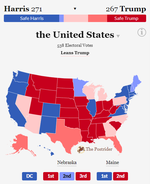
The rating for the entire race still said “Lean Trump” and the map clearly leans Trump, but Kamala Harris still nets a winning 271 electoral votes… 

This isn’t as confusing as it seems – the reason for this is that Harris just has a lot more “safe” states in this scenario, and comparatively few lean or likely states, whereas Trump has a lot electoral votes stuck in lean or likely states. Now, what the model did at this stage was assign a 60% probability of a win (and 60% of electoral votes) to every lean state, and an 85% probability to every likely state. Texas and Florida – both likely Trump here – are the second- and third-largest states, respectively, worth 70 combined electoral votes, and Harris was getting about 10 electoral votes from them just because the model was hedging against the outside risk she overperformed. In all of the lean states, Trump was getting only 60% of their electoral votes, and Harris 40%. But with very few lean or likely states on the blue side, the model was just giving Harris an extra boost here. This is a result of our step function that had hard cutoffs for when states were considered toss-up, lean, likely, or safe – any state between D+5 and D+10, whether D+5.1 or D+9.9, was getting an 85% chance applied to it.

There’s an argument that this – though confusing – isn’t that bad: the model is suggesting Harris has way more electoral upside than Trump and a chance to do better overall. That’s probably true. It’s also being very careful, because it is a very conservative model at the center: assigning very few electoral votes (or Senate seats, in the Senate model) to races where a party only has a slim lead. This worked out for us really well in 2022 and 2020, especially compared to FiveThirtyEight or The Economist, as our ratings were being much more cautious about the projected total.

But it also contradicts what we know about Electoral College bias, which is that the electoral map narrowly favors Trump because the tipping point state is likely a couple points to the right of the nation overall. And, no matter what, it’s not giving a good probability breakdown. It needs a fix.

The good news is the problem is just in the topline forecast, essentially just the last “part” of the model – but it’s also probably the part that matters the most to you, unless you’ve really liked playing along with our interactive model!

A Normal Solution

Start with what we were getting right: a clear strength of our model is this conservatism in the middle ranges and a more aggressive assertion of safety at the extremes. This protected us against big polling errors in 2020, for example, but made our model more grounded at the extremes. A solution should look like this, but be smoother, jumping less aggressively in its assignment of odds from a D+4.9 state to a D+5.1 state – this demanded a bit more mathematical rigor.

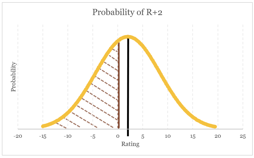
The best way to do this is with a normal distribution, giving us a probability of a certain party winning a state given its final rating. Put otherwise, if the state is R+2, what’s the probability it goes for the Republican instead? 

Our step function worked historically because it protected us if we were a bit off in a state. The problem is now our model is giving a rating given a generic ballot position, so it can adjust over time. These two things are obviously related (if the generic ballot polls are off by D+3, you might expect state polls to also be off by around D+3), so we’ll need to consolidate and find a solution that catches the degree of risk in both. 

To get a normal distribution for every given point, we pulled the average polling error data for each Senate and presidential cycle from 2000 to 2022, which had a mean of 4.789 and a standard deviation of 0.743; by dividing the mean by the standard deviation we can reconcile those into a standard deviation which is inclusive of the average polling miss, about 6.45. From this standard deviation, we can run a normal distribution on top of any given rating, then just calculate the probability of all of the area below the “zero” point.

For example, given a rating of R+2, we can drop a normal distribution with that standard deviation on top of it, and then use R+0 as the probability calculation point – calculating just the probability that there is an outcome resulting in a Democratic win (only the area under the curve below zero). For R+2, there is about a 38% chance that the Democrat will win. 

We can derive a cumulative distribution function from this for each given rating:

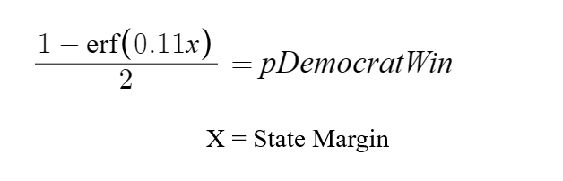
Using this, we have a smooth, steady, relatively conservative probability distribution for given ratings. We can still be very cautious with how we weigh a D+2 or D+3 state (62% and 68% chances of Democratic victory, respectively), but also acknowledge that D+9 is meaningfully more Democratic-leaning than D+5.5 (92% chance and 80% chance, respectively).

Implementation and Adjustments

By switching out our step function for this cumulative distribution function, the forecast is much more smooth: states aren’t aggressively ratcheting up the percent chance of a win based on small movements, and we’re still being very careful and conservative in awarding votes in a tight race.

The projected Electoral College totals are now calculated by using this function, but awarding electoral votes similarly (if Harris has a 68% chance of winning a state with ten electoral votes, then she will get 6.8 electoral votes and Trump will get 3.2). Same goes for Senate seats – an 81% chance of winning a Senate race nets that party 0.81 seats, and the opposing party 0.19 seats.

This requires a few methodological and visual adjustments too. Our qualitative descriptors of ratings (as in, what determines if something is called “safe” or “lean”) will also stay the same, though the points at which they’re implemented have shifted according to this new function: 

• Toss-up will still be any state with less than 60% chance of going to any party (roughly between R+1.6 and D+1.6)
• Lean will have between a 60% and 85% chance of going to any party (roughly between R+1.6 and R+6.7)
• Likely will have between an 85% and 98% chance of going to any party (roughly between R+6.7 and R+13.3)
• Safe will any race with greater than a 98% chance of going to any party (greater than R+13.3)

We have also added the probability of each race, to really showcase that not every “lean” or “likely” state is being treated equally, and give the odds of the favored party.

The United States Rating

Finally, for the United States’ rating, we’ve added one more level of probability to adjust for any national generic ballot error and to give a final probability for the party favored to win the White House or the Senate. 

For the presidential model, we first take the estimated electoral votes given the current generic ballot rating. Second, we find what the generic ballot would need to be for the Republican electoral votes to be 268 (we use 268 instead of 269 because, frankly, Trump is heavily favored to win a contingent election in the House of Representatives, should a tie occur). 

For the Senate model, we first take the estimated number of Senate seats given the current generic ballot. Second, we find what the generic ballot would need to be for the number of Republican Senate seats to be less than the seats required for victory (in 2024, they need to win 13 seats to get 51 senators), then we run a check to verify that at that generic ballot the odds of the presidential race going to the Democrat are higher than 50% (this cycle, this is essentially a given, as the Senate map overwhelmingly favors Republicans).

Then – for both – we run a normal distribution given the current generic ballot, the “tipping point” generic ballot, and the standard deviation for national generic ballot errors using data from the 21st century (about 2.64). The cumulative probability here tells us the percent chance that Democrats have of winning the presidency or the Senate.

It’s important to be very clear about what exactly is being predicted (some shade intended), so let’s put this clearly:

• An individual state’s rating and probability are based on the odds a state has of being won by a given party.
• The United States’ rating and probability are based on the odds that a given party will win the national contest: the Electoral College, in the case of the presidential model; a majority of Senate seats, in the case of the Senate.

And that should do it! Our methodologies have been updated accordingly, of course. We’ll be in touch again soon with some state-level updates, and as the models finish getting filled out. As always, if you have any questions, suggestions, or feedback, just let us know!